Get started
STEEL is an unsupervised algorithm based on manifold learning to analyze spatial transcriptome data. It presents strong and robust performance on revealing the distribution of different types of cells in various tissues.
STEEL is implemented in C++ to promote computing speed for spatial transcriptome analysis.
Obtaining STEEL
The newest version of STEEL is available at SourceForege
System requirement
- 64-bit operating system
- 10G bytes memory *
- C++ compiler *
Please note that the memory size required is proportional to square of bead number.
Installation
Installation from source code
g++ src/STEEL.cpp -o steel -O3
Executable files for 64-bit linux and mac OS have already been included
- steel_linux64
- steel_macos
Then move a executable file to your PATH
Running STEEL
Running STEEL on 10X Visium data
A folder and a file are required for analyzing 10X Visium data:
- a folder including three files with FIXED names:
- barcodes.tsv
- features.tsv
- matrix.mtxs
- a file for bead location on slides, usually with name as:
- tissue_positions_list.csv
usage:
steel express_folder space.csv out_prefix
Running STEEL on Slide-seq data
Two input files are required for analyzing slide-seq data:
- a file for gene expression of beads, for example:
- Puck_200115_08.digital_expression.txt
- a file for bead location on slides, for example:
- Puck_200115_08_bead_locations.csv
typical format of *.digital_expression.txt
GENE    AACGTCATAATCGT  TACTTTAGCGCAGT  CATGCCTGGGTTCG  TCGATATGGCACAA
0610005C13Rik   0   0   0   0
0610007P14Rik   1   0   0   2
0610009B22Rik   1   0   2   0
0610009E02Rik   0   0   0   0
0610009L18Rik   0   0   0   0
0610009O20Rik   1   0   0   0
0610010F05Rik   2   0   3   1
0610010K14Rik   0   0   0   0
0610011F06Rik   5   2   2   3
typical format of *_bead_locations.csv
barcodes,xcoord,ycoord
AACGTCATAATCGT,888.95,3219.5
TACTTTAGCGCAGT,4762.2,5020.4
CATGCCTGGGTTCG,886.5,3199.6
TCGATATGGCACAA,2237.1,5144.6
TTATCTGACGAAGC,1031.8,2425.2
GATGCGACTCCTCG,5387,2291.6
ACGGATGTTCCGAT,3760.3,4171.7
TCTCATGGGTGGGA,1007.9,3523.8
ACCGGAACTTCTTC,3259.4,1233.7
usage:
steel express.csv space.csv out_prefix --data=slide-seq
in case of the two files adopting alternative separators (e.g. comma), run:
steel express.csv space.csv out_prefix --data=slide-seq --sepe=comma
steel express.csv space.csv out_prefix --data=slide-seq --seps=comma
Running STEEL on MERFISH data
A single file is required for analyzing MERFISH data:
- a file for gene expression of beads, for example:
- merfish_all_cells.csv
- an option for specifying animal ID and layer (comma-separated), for example:
- 1,0.01
typical format of merfish_all_cells.csv
Cell_ID,Animal_ID,Animal_sex,Behavior,Bregma,Centroid_X,Centroid_Y,Cell_class,Neuron_cluster_ID,Ace2,Adora2a,Aldh1l1
e9d73818-5233-41aa-b387-25257543d9de,18,Female,Parenting,0.26,-3022.004661,-913.4363878,Inhibitory,I-17,0,0,2.635883841
704470b6-2455-4e8d-be4c-6337b017efd0,18,Female,Parenting,0.26,-3020.644809,-999.3269277,Inhibitory,I-17,0,3.77199522,0
16b60d1b-e1b9-40e3-bd99-848f2c03047a,18,Female,Parenting,0.26,-3017.659617,-981.6438722,Inhibitory,I-17,0,0,0
f5346407-1501-407d-b981-445f46023b16,18,Female,Parenting,0.26,-3016.583112,-968.2165641,Inhibitory,I-17,0,1.008907777,0
b1ab923f-d5fd-4eff-99d3-76bb333db9b2,18,Female,Parenting,0.26,-3014.546591,-951.9463638,Inhibitory,I-17,0,19.7826058,1.098939884
52575404-3e6b-4d81-9e4a-e0e4258eab8e,18,Female,Parenting,0.26,-3012.963751,-933.8142342,Inhibitory,I-17,0,0,1.111835081
58e45f88-dd85-42cc-aecb-fad5c7319681,18,Female,Parenting,0.26,-3009.642496,-872.2212331,Inhibitory,I-17,0,0.677915168,0.677915168
e099f612-ee04-4c04-807d-717e9d3b9bcf,18,Female,Parenting,0.26,-3009.086423,-889.4591559,Inhibitory,I-17,0,1.779969301,1.779969301
8ec89fed-6a19-4923-b5ad-bd4eae15d608,18,Female,Parenting,0.26,-3008.514393,-996.2985381,Inhibitory,I-17,0,6.347845229,2.380492681
usage:
steel merfish_all_cells.csv 18,0.26 out_prefix --data=merfish
Running STEEL on STARmap data
A folder (for expression info) and a file (for spacial info) are required for analyzing STARmap data:
- a folder including three files with FIXED names:
- cell_barcode_names.csv
- cell_barcode_count.csv
- a file for bead location on slides, usually with name as:
- centroids.tsv (made based on "labels.npz" according to the manual of STARmap)
typical format of cell_barcode_names.csv
0,311412,1110008F13Rik
1,424121,1110008P14Rik
2,224433,1700019D03Rik
3,313212,1700086L19Rik
4,211112,2810468N07Rik
5,321213,2900055J20Rik
6,134413,2900092D14Rik
7,121143,3110035E14Rik
8,324221,3632451O06Rik
9,314424,6330403K07Rik
typical format of cell_barcode_count.csv
0,1,0,0,0,0,0,0,0,0,0,1
0,0,0,0,0,0,0,0,0,0,0,0
1,0,0,2,0,0,0,0,0,0,0,0
0,0,0,0,0,0,0,0,0,0,0,0
0,0,0,0,0,1,0,0,0,1,0,0
0,2,0,1,0,0,0,1,0,0,0,0
0,0,0,0,0,0,0,0,0,0,0,1
0,0,0,0,0,0,0,0,0,0,0,0
0,0,0,0,0,0,0,0,0,0,0,0
0,0,0,1,0,0,0,1,1,0,0,0
typical format of centroids.tsv
19.918240442192538  1951.6273606632888
27.798811396608983  2969.047718930257
26.73331096947333   2804.8455216370344
24.085884205002625  8867.800069966766
26.384917517674783  10853.26207776905
34.105634933376145  1160.4862738802376
35.575841452612934  866.5514836138175
36.09220423979941   2300.663779348074
49.77124718410813   4980.7776640043685
53.473113918182875  8729.177424962336
usage:
steel express_folder centroids.tsv out_prefix --data=starmap --gini=0.4 --pca=5
in case of the two files adopting alternative separators (e.g. comma), run:
steel express.csv space.csv out_prefix --data=slide-seq --sepe=comma
steel express.csv space.csv out_prefix --data=slide-seq --seps=comma
Parameters
--data=: data type, [10X-ST/slide-seq/merfish/starmap], default: 10X-ST--perp=: perplexity for inferring variation from expression matrix, default: 35--k=: number of neighbors for inferring radius, default: 20--beads=: minimal bead percent for each gene, default: 0.0005--genes=: minimal gene percent for each bead, default: 0.005--group=: min,max output group number , default: 20,40--gini=: minimal spatial Gini coefficient, default: 0.5--hvg=: a file for user defined highly variable genes (HVGs). This option overwrites that of Gini coefficient.--exclude=: a file for excluded genes (mitochondrial genes)--min_read=: minimal read number per bead per gene, default: 1--pca=: num of principal components, ZERO for ignoring PCA, default: 0--sepe=: separate character for input expression matrix of slide-seq, could be tab/space/comma, default=comma--seps=: separate character for input space matrix of slide-seq, could be tab/space/comma, default=comma--all_genes=: output expression of groups for all genes, default: F
Output format
- output_prefix.map.*: clustering results of beads, tabular format with four columns:
- bead name
- x coords
- y coords
- group
an example:
Bead    x   y   Cluster
AAACAAGTATCTCCCA-1  50  102 1
AAACACCAATAACTGC-1  59  19  17
AAACAGAGCGACTCCT-1  14  94  20
AAACAGCTTTCAGAAG-1  43  9   19
AAACAGGGTCTATATT-1  47  13  19
AAACATGGTGAGAGGA-1  62  0   9
AAACATTTCCCGGATT-1  61  97  35
AAACCGGGTAGGTACC-1  42  28  22
AAACCGTTCGTCCAGG-1  52  42  16
- output_prefix.genes.*: predicted marker genes, tabular format with columns as:
- gene name
- group ID
- gini score
- p-value
- q-value
- bead num in groups
an example:
Gene    Marker  Score   p_value q_value G1  G2  G3  G4  G5
ENSMUSG00000061808  5,7,33  0.948211    0.000570247 0.0020117   1.80662 3.29322 0.555393    1.39566 8.15028
ENSMUSG00000001023  9   0.911682    4.68554e-27 1.40015e-25 0   0   0.485622    0   0
ENSMUSG00000026051  5,7 0.859619    7.52768e-69 4.78007e-67 0.0256069   0.0891366   0.354038    0   1.79188
ENSMUSG00000024871  9,10,11,12,16,17,18,19,26   0.853481    1.74714e-11 1.43153e-10 0.0226423   0.0273269   0.302561    0.0566058   0
ENSMUSG00000021803  9,10,11,12,17,18    0.836802    6.33667e-12 5.45598e-11 0.0113212   0   0.0528321   0   0
ENSMUSG00000096883  19  0.81827 0.000738979 0.00255124  0.0113212   0.0546539   0.105664    0   0.0440267
ENSMUSG00000000214  9,10,11,17,18,19    0.809173    3.20513e-15 3.97124e-14 0   0   0.0528321   0   0
ENSMUSG00000003657  9,10,11,12,17,18,19 0.80577 2.79267e-07 1.57631e-06 0.122236    0.0273269   0.172331    0.257131    0.0440267
ENSMUSG00000041911  9,10,11,17,18,19    0.795939    8.22408e-13 7.88271e-12 0   0.0718953   0   0   0.111111
Visualizing in R
#load data ("*.map.10" denotes for 10 groups clustering)
data=read.table("results/output.map.10", header=T, row.names = 1)

#plot spatial clustering results using user-defined color palette
plot(data[,1:2], col=color_palette[data[,3]], pch=16)
Examples
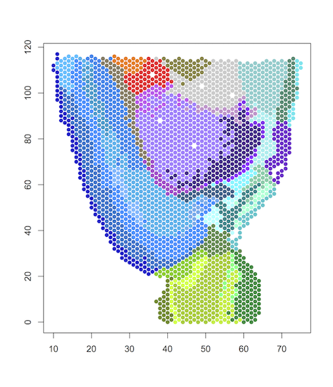
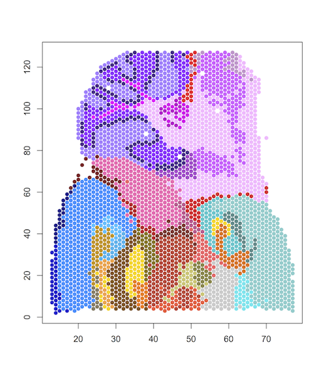
Mouse brain datasets (sagittal plane) of 10X Visium
Data availability
The spatial transcriptomic datasets are available on the official website of 10X Genomics
Clustering data using STEEL
# a mouse brain dataset (anterior section on sagittal plane)
steel Sagittal_Anterior_Section_0 Sagittal_Anterior_Section_0/tissue_positions_list.csv anterior --exclude=mito.genes.10Xid

# a mouse brain dataset (posterior section on sagittal plane)
steel Sagittal_Posterior_Section_2 Sagittal_Posterior_Section_2/tissue_positions_list.csv posterior --exclude=mito.genes.10Xid
The option --exclude=mito.genes.10Xid is for removing mitochondrial genes from the expression matrix.
The names of these mitochondrial genes are available at Mouse Genome Informatics and are also distributed with STEEL.
Visualization in R
#load data
data=read.table("results/anterior.map.41", header=T, row.names = 1)

#plot spatial clustering results using user-defined color palette
plot(data[,1:2], col=color_palette[data[,3]], pch=16)
#load data
data=read.table("results/posterior.map.41", header=T, row.names = 1)

#plot spatial clustering results using user-defined color palette
plot(data[,1:2], col=color_palette[data[,3]], pch=16)
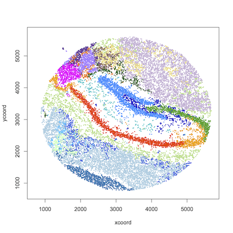
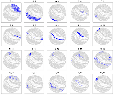
Mouse brain datasets (hippocampus) of Slide-seq
Data availability
The spatial transcriptomic datasets of Slide-seq are available on Broad institute’s single-cell repository
- hippocampus (Puck_200115_08)
- olfactory bulb (Puck_200127_15)
Clustering data using STEEL
# a hippocampus dataset
steel Puck_200115_08.digital_expression.txt Puck_200115_08_bead_locations.csv hippocampus --exclude=mito.genes --data=slide-seq

# an olfactory bulb dataset
steel Puck_200127_15.digital_expression.txt Puck_200127_15_bead_locations.csv olfactory --exclude=mito.genes --data=slide-seq --min_read=0 --genes=0.01
The option --exclude=mito.genes is for removing mitochondrial genes from the expression matrix.
The names of these mitochondrial genes are available at Mouse Genome Informatics and are also distributed with STEEL.
Visualization in R
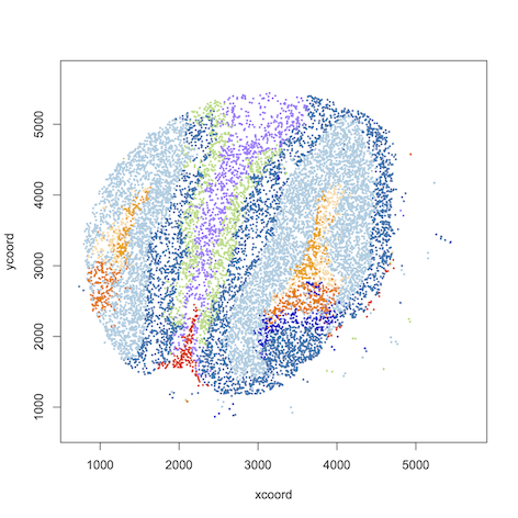
#load data
data=read.table("results/hippocampus.map.20", header=T, row.names = 1)

#plot spatial clustering results using user-defined color palette
plot(data[,1:2], col=color_palette[data[,3]], pch=16)
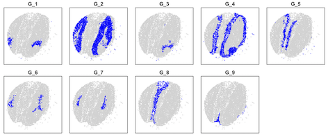
layout(matrix(1:20,4,5,byrow = T))
par(mai=c(0.1,0.1,0.2,0.1))
for(i in 1:20) {
  plot(data[,1:2],col="lightgray",pch=16,cex=0.2,xlim=c(700,5700),ylim=c(700,5700),xlab=NA,ylab=NA,yaxt="n",xaxt="n",main=paste("G_",i,sep=""))
  points(data[data[,3]==i,1:2],col="blue",pch=16,cex=0.2,xlim=c(700,5700),ylim=c(700,5700))
}
#load data
data=read.table("results/olfactory.map.9", header=T, row.names = 1)

#plot spatial clustering results using user-defined color palette
plot(data[,1:2], col=color_palette[data[,3]], pch=16)
layout(matrix(1:10,2,5,byrow = T))
par(mai=c(0.1,0.1,0.2,0.1))
for(i in 1:9) {
  plot(data[,1:2],col="lightgray",pch=16,cex=0.3,xlim=c(700,5700),ylim=c(700,5700),xlab=NA,ylab=NA,yaxt="n",xaxt="n",main=paste("G_",i,sep=""))
  points(data[data[,3]==i,1:2],col="blue",pch=16,cex=0.3,xlim=c(700,5700),ylim=c(700,5700))
}
Mouse brain datasets (hypothalamus) of MERFISH
Data availability
The spatial transcriptomic datasets of MERFISH are available on (https://datadryad.org/stash/dataset/doi:10.5061/dryad.8t8s248)
- hypothalamus (Moffitt_and_Bambah-Mukku_et_al_merfish_all_cell)
Clustering data using STEEL
# layer 0.26 from sample 18 from the hypothalamus dataset
steel Moffitt_and_Bambah-Mukku_et_al_merfish_all_cells.csv 18,0.26 sample18_0.26 --data=merfish --group=5,20
Visualization in R
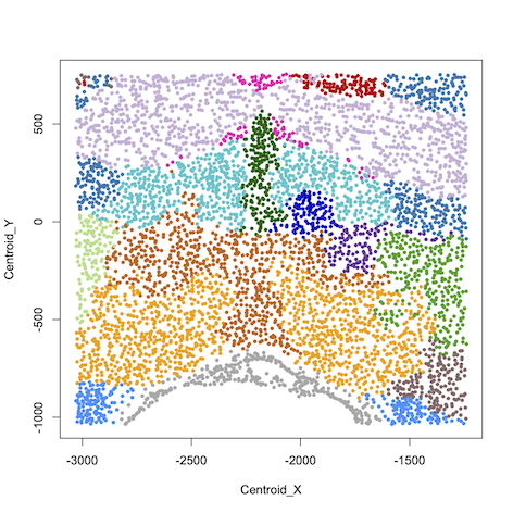
#load data
data=read.table("results/sample18_0.26.map.15", header=T, row.names = 1)

#plot spatial clustering results using user-defined color palette
plot(data[,1:2], col=color_palette[data[,3]], pch=16)
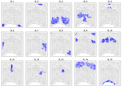
layout(matrix(1:15,3,5,byrow=T))
par(mai=c(0.1,0.1,0.2,0.1))
for(i in 1:15) {
  plot(data[,1:2],col="lightgray",pch=16,cex=0.4,xlab=NA,ylab=NA,yaxt="n",xaxt="n",main=paste("G_",i,sep=""))
  points(data[data[,3]==i,1:2],col="blue",pch=16,cex=0.4,xlab=NA,ylab=NA)
}
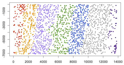
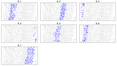
Mouse brain datasets (visual cortex) of STARmap
Data availability
The spatial transcriptomic datasets of STARmap are available on (https://www.starmapresources.com/data)
- visual cortex (20180505_BY3_1kgenes)
Clustering data using STEEL
# a visual cortex dataset
steel 20180505_BY3_1kgenes 20180505_BY3_1kgenes/centroids.tsv by3_1kgenes --data=starmap --gini=0.4 --pca=5 --group=5,20
The option --gini=0.4 is for utilizing spatially varying genes with Gini coefficient >= 0.4.
The option --pca=5 is for employing the top 5 PCA components for clustering.
Visualization in R
#load data
data=read.table("results/by3_1kgenes.map.7", header=T, row.names = 1)

#plot spatial clustering results using user-defined color palette
plot(data[,1:2], col=color_palette[data[,3]], pch=16)
layout(matrix(1:9,3,3,byrow=T))
par(mai=c(0.1,0.1,0.2,0.1))
for(i in 1:7) {
  plot(data[,1:2],col="lightgray",pch=16,cex=0.5,xlab=NA,ylab=NA,yaxt="n",xaxt="n",main=paste("G_",i,sep=""))
  points(data[data[,3]==i,1:2],col="blue",pch=16,cex=0.5,xlab=NA,ylab=NA)
}
Contributors
Developed by Yamao Chen, Shengyu Zhou, Ming Li, Fangqing Zhao and Ji Qi
Acknowledgement
- Thank the eigen-core-team for providing Eigen, a C++ template library for linear algebra.
- Thank Dr. Kasper Peeters for providing [tree.hh], which is a C++ class for tree construction/operation and available at GitHub.
- The availability of a C++ class [StringTokenizer.h] by Dr. Christiane Lemke is also highly appreciated.